Drilling Optimazation

ROP simulation using Generative Deep Learning

Drilling and Eploration

Is one of the fields where tonnes of data are collected daily. It is also one of the areas where applying Machine Learning and AI can bring significant benefit making it faster, cheaper, efficient and safer.

Objectives and Goals

The purpose of the study is to analyze the performance and drilling efficiency of a given well, as well as model ROP using Generative Machine Learning Techniques:

► estimate drilling efficiency using statistics;
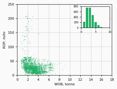
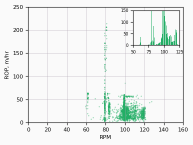
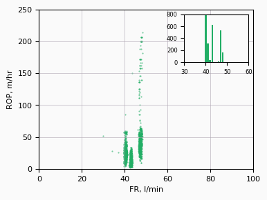
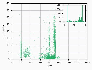
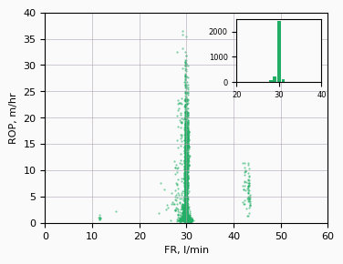
► analyze the correlation between ROP and Drilling Parameters;
► model ROP in different drilling scenarios using Machine Learning.

Dataset

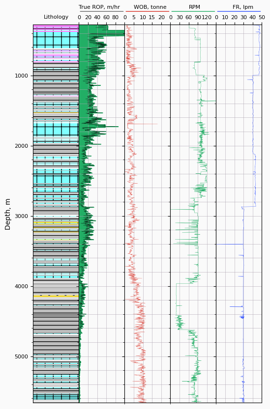
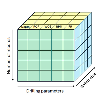
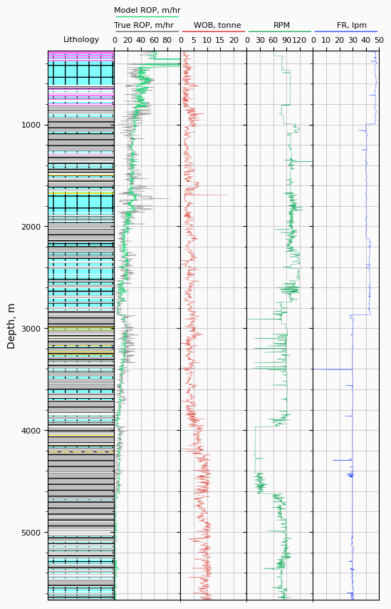
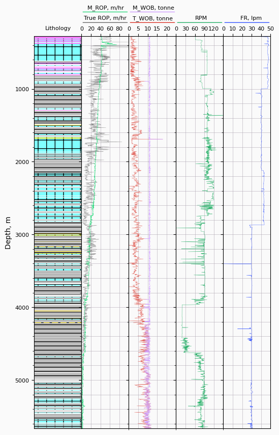
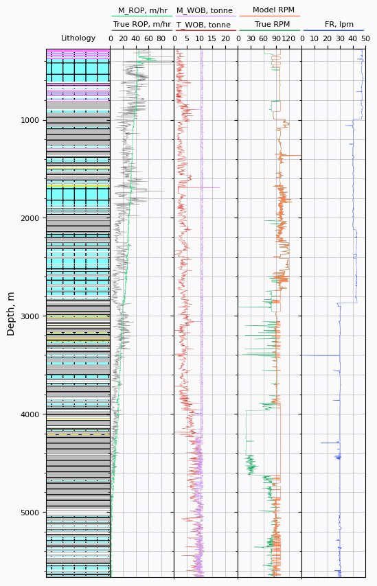
The dataset that was used for this study consists of the following parameters:

● Depth - Measured Depth
● ROP - Rate of Penetration
● WOB - Weight on Bit
● RPM - Rate per Minute
● FR - Flow Rate

2. Key Insights and Observations

12.25" Section

✓Overall good performance in 12.25" section;
✓Low WOB (< 8 tons) was applied, which can be a subject for optimization on the next wells;
✓Rotary BHA was used, which can be seen from the WOB and ROP correlation;
✓RPM is normally distributed around the 100rpm;
✓FR data can be broken down into 3 clusters, which indicates that it was adjected accordingly as the section progressed.

8.5" Section

✓Relatively good ROP in the upper part of the sections (up to 4200 m), where formation is mostly soft and medium;
✓Starting from 5000 m the formation becomes hard, which indicates overall low (< 2 m/hr) ROP, despite the high (around 10 tons) WOB applied;
✓Drilling parameters, BHAs and drill bits optimization are essential to improve performance in bottom part of the section;
✓Different types of BHA was used (Rotary and Mud Motor), which can be deduced for RPM distibution;
✓FR was barely adjusted.

3. Model Architecture

The generative model used in this project is a variation of the Diffusion Model. The main objective is to train the network to denoise the ROP by learning to represent it in terms of other drilling parameters.

We treat the sequential, depth-based drilling data as a collection of small images (5 x 5 in our case). To achieve this, the entire dataset is sliced into overlapping 5 x 5 matrices, shifting by 1 step (1 meter) downward. Given that our dataset consists of 5,402 points, this results in 5,397 slices.

Next, we add random noise to the ROP and feed the resulting 3D tensor into our model, as shown below.

Slice dataset

1817	22.05	1.61	97.11	40.84
1818	22.55	1.87	98.82	41.02
1819	22.30	1.61	96.21	40.84
1820	22.14	1.41	94.61	40.84
1821	23.52	1.60	95.98	40.80

Add random noise to ROP

→

Combine data

To simulate different drilling dynamics, we simply replace the actual drilling parameters (WOB, RPM, and FR) with desired values while keeping the ROP unchanged, with the same amount of noise added.

5. Conlcusions and Recomendations

✓ Simulation shows that incresing WOB tends to improve drilling perfomance and increase overall ROP.
✓ Running Mud Motor BHA and applying high FR in soft foamtion is benefitcial for incresing ROP.
✓ Managing drill bit aggressiveness and optimizing hydraulics are key to maximize ROP in soft and medium formation.
✓ Improvement of drill bit technology and designs are essential for drilling lower part of 8.5" section.

ROP simulation using Generative Deep Learning

Drilling and Eploration

Objectives and Goals

Dataset

1. Drilling Efficiency Estimation

Driling Parameters

12.25" section (from 0 m to 2500 m)

ROP vs WOB

ROP vs RPM

ROP vs FR

8.5" section (from 2500 m to 5670 m)